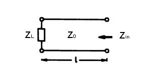
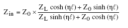
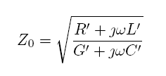
Transformation of the impedance ZL into impedance Zin by a two-wire line with the (complex) impedance Z0 of the length l.
At the simulation of (vertically) aerials there are two determining factors: The conductivity and relative permittivity of the ground with high frequency (short soil conductivity). However, exactly these values are, up to now, only raw estimates or taken out of the easiest maps for long-wave transmitter and medium-wave radio stations. Information for the short wave band is not to be found at all. Besides, the ground qualities are dependent very much on the frequency. Hence, I would like to observe these values for a longer period together with the amount of precipitation and temperature myself.
The ground qualities can be measured with the shown procedure easily at several places for all desired frequency. The measurement refers of course only to the uppermost layer in that the two-wire line is introduced. With a rock ground with 40 cm of humus in the flowerbed measured, this measurement does not show the average of the surroundings! However, with care at the estimations very useful results are absolutely to be achieved.
At last these values serve for the comparison of two ground plane aerials with raised resonant radials or buried radials in the simulation with NEC4.2 as well as with a detailed measurement.
A two-wire line is introduced in the ground and the impedance is measured as a vector at the upper end. The two-wire line in the ground is open at the lower end. The two-wire line transforms this impedance as a function of her geometrical qualities and the qualities of the medium (surface of the earth). The general two-wire line equation is used to determine the relative permittivity εr and the specific conductivity σ.
Transformation of the impedance ZL into impedance Zin by a two-wire line with the (complex) impedance Z0 of the length l.
Is worth
 with
with
Because the two-wire line is open at the end we choose for ZL a still to be determined value which considers the fringing effect of the two-wire line.
Here, you can read about an approximation of the fringing effect of a two-wire line.
The following applies to such a two-wire line
 .
.
The primary line constants are:
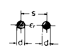
C' = ε0 * εr * π / acosh(s/d)
L' = µ0 * µr / π * acosh(s/d) ; [1]
G' = σ * π / acosh(s/d)
R' = 1,66 * 10-7 * K1 * √f / d ;with simplification after [2] for this rigid wire line
---------------------
[1] µr at high frequency (~1.0 in the whole HF area, also with magnetic mild steel)
[2] Janzen, Gerd: Kurze Antennen : Entwurf u. Berechnung verkürzter Sende- und Empfangsantennen, 1986, ISBN 3-440-05469-1
| metal | K1 |
| aluminum alloyed | 1,3 - 2,0 |
| copper | 1,0 |
| brass | 1,9 - 2,3 |
| zinc | 1,9 |
| steel | 2,8 - 3,6 |
| stainless steel | 7,2 |
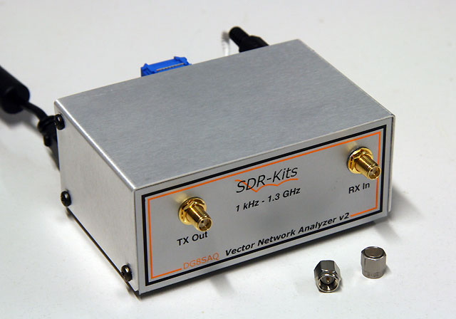
With the new vector network analyzer of DG8SAQ an exact analysis is possible for every amateur.
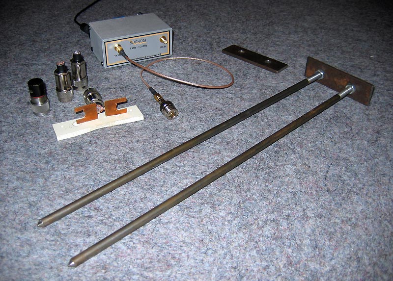
All parts required to the measurement.
The mechanical dimensions of my two-wire line are d = 8.0 mm s = 48.0 mm l = 400 mm
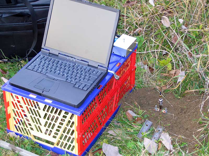
Measurement with laptop, vector network analyzer of DG8SAQ and two-wire line in the ground.
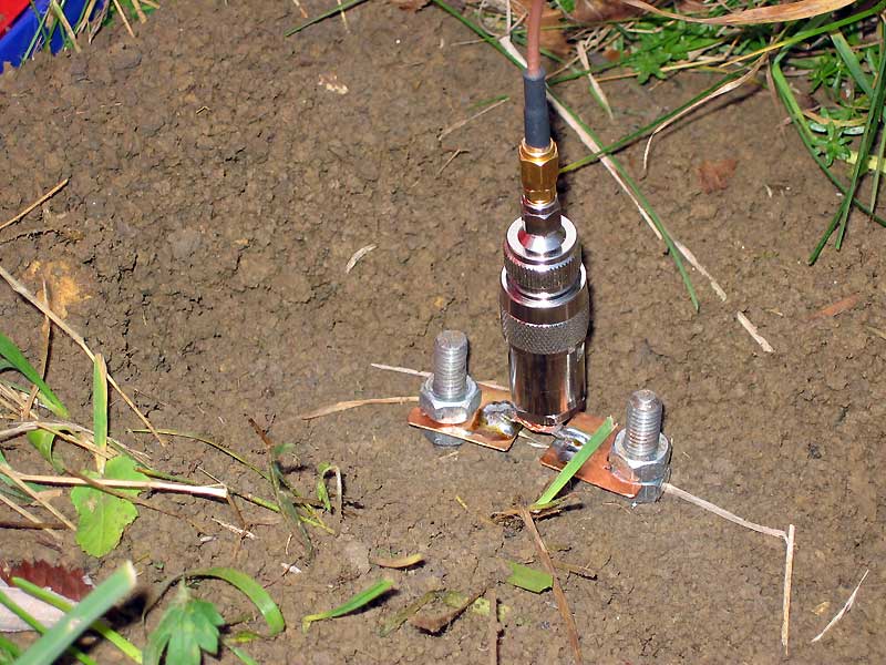
End of the two-wire line in the ground with adapter and coaxial cable.
The two-wire line to be introduced in the ground exists here of two iron rods with 8 mm of diameter and 40-cm length. Both poles have a thread at the upper end and the lower end is sharpened to make it easier to press it into the earth.
One of both steel-plates with two holes lie on the ground and serves for stabilization of the distance of the poles. The other record is screwed together at the upper end on nuts. Then, the poles are fastened together like shown in the picture. Then, the rod assembly is to be pressed into the earth. If the two-wire line is completely in the ground both steel-plates are removed and the adapter piece (here with N plug) is screwed on, and the measurement is carried out. For the adapter piece, two conformist calibrating standards are built to allow a SOL calibration. The poles can be also pulled out of the ground one after the other very easily by using the steel-plate.
Don't forget to think about a BalUn between your analyzer and the symmetrical two wire line. Or your structure is floating, and the connection line is very short like mine.
The conversion of the measured impedance into the specific permittivity εr
and the specific conductivity σ of the ground is done with a numerical solution.
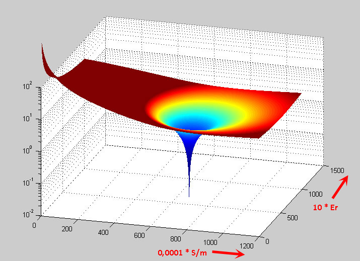
The solution of the equation may result in very nice pictures.
In the picture the divergence of all possible solutions is shown.
The X and Y axes stretch the level of all possible qualities εr and σ.
The ground characteristic can be calculated with my self-developed computer program:
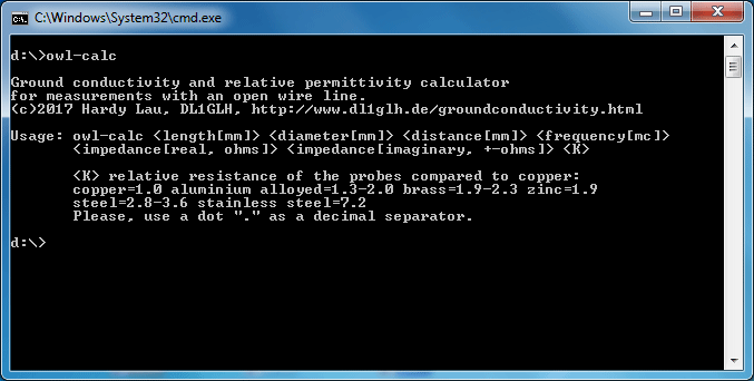
Start of the program in the windows console without parameters.
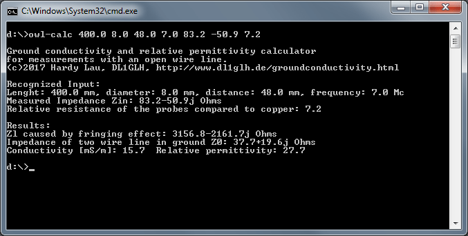
Start of the program with parameters and the printed result.
Here you can download the program owl-calc with sources (GPL V3) for offline use (Microsoft Windows).
The numerical solution is done with "C" (MinGW with GCC) and also with MATLAB.
By the general two-wire line equation all mechanical dimensions are possible, as long as the two-wire line is electrically no longer than 1/2 λ. The calculation is no simple approximation but an exact solution. The dimensions orientate themselves by the possible mechanics and the precision of the measuring instrument.
The plausibility of the conversion into the earth properties was checked quite several times successfully. With a high conductivity the measurement also occurs in the right depth because the current penetration depth becomes already very small. If necessary the means from several measurements must be taken in the sphere of the aerial up to several λ distance.